Visualizing Videos with Python
The next best thing to printing a gif. —
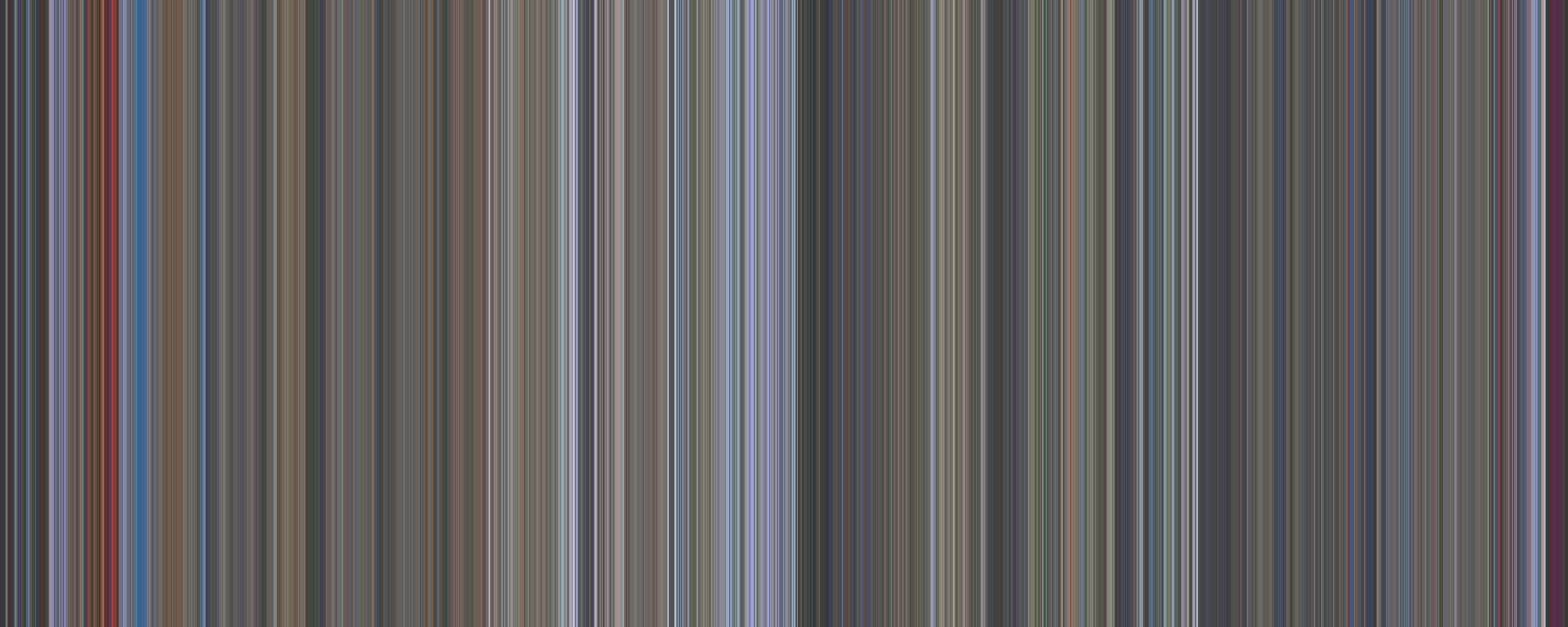
A visualization of The Net (1995).
I’m a big fan of movies, not necessarily cinema mind you, my taste is nowhere near refined enough for that, but I have a huge respect for anyone able to put their vision out into the world and love seeing those ideas in any form they take. So last year, I was entranced when I saw an ad for the hybrid of technology and art that is the “Frome”. The official site describes them well:
The canvases you see are movies condensed into chronological color strips that represent each frame - meaning the colors you see can roughly represent the main color of that scene. The movie begins with a single color strip at the start of canvas (left) and ends with the last strip (right). You can see how beautiful movies are in terms of colors!
I really liked the idea of one of their canvases sitting in my living room, but:
- The canvases don’t come in the sizes I want.
- Their selection is geared more toward cinema, and if I want Birdemic on my wall, I should be allowed to have it!
From my work building an image to cross-stitch pattern generator for my wife I knew that K-means was good at picking out representative colors from a static image so I figured it would do fairly well on videos as well. If you’re not interested in the tuning, you can skip to the bottom for the code.
Adventures in OpenCV land
At first, I tried clustering RGB, but everything was coming out wonky. Reading closely through the OpenCV code, it turns out that they use BGR, not RGB for historical reasons so when I was converting that to hex the blue and red channels were getting flipped. When clustering, I swapped colors to HSV space because it was better at preserving vibrancy of colors and made the outputs less muddy.
I also tried adjusting K up and down, and five seemed to be a sweet spot. But, it’s art so tune the hyperparameter to something that makes you happy rather than aiming for something publishable.
With that fixed, I finally started to get some nice images, but things were slow on larger films. I first cut down the frame size dramatically to decrease the number of pixels that K-means had to operate on then chose to only pick out one frame a second. Frome claims to do one strip per frame, but at 90+ minutes, a feature length film shot at a standard 24 FPS would be at least 129600 pixels. Printing that out at 300 PPI would be over 30 feet wide, so I decided I could afford to downsample to only one frame a second.
Conclusion
At the end, I got something that looks like the hero image for this article. Comparing the official versions to mine yield similar results with a couple of caveats. The image below is for Pan’s Labyrinth (2006):
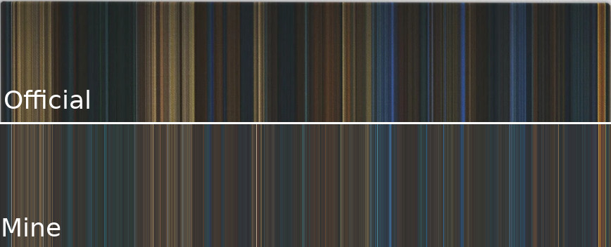
Their colors definitely pop better, so they might have done post-processing or adjusted their algorithm for color richness. The official ones are also a bit less stripey which might be an artifact of theirs being printed on a canvas, greater downsampling, or some kind of temporal cohesion going on. I suspect seeding one round’s K-means starting values with those from the previous frame might smooth out some of the random stripes.
Code listing
import numpy as np
import cv2
from sklearn.cluster import KMeans
import math
import os

SKIP_FRAMES = 24 # Capture 1 in every SKIP_FRAMES frames, usually films are 24 FPS.
NCOLORS = 5 # Number of colors to use in k-means.

video = "0001.mp4" # Movie file to load.

base = os.path.basename(video)
base = os.path.splitext(base)[0]

cap = cv2.VideoCapture(video)
total_frames = cap.get(cv2.CAP_PROP_FRAME_COUNT)

colors = []
frame_num = 0
while(cap.isOpened()):
    ret, frame = cap.read()
    if not ret:
        break # Likely end of file.

    # Speed up computation by skipping frames.
    frame_num += 1
    if frame_num % SKIP_FRAMES != 0:
        continue

    # Speed up computation by reducing size of the frame to 1/10th on each side.
    tinyframe = cv2.resize(frame, None, fx=.1, fy=.1, interpolation=cv2.INTER_AREA)

    # Convert to HSV color space.
    tinyframe = cv2.cvtColor(tinyframe, cv2.COLOR_BGR2HSV)

    pixels = np.float32(tinyframe.reshape(-1, 3))
    criteria = (cv2.TERM_CRITERIA_EPS + cv2.TERM_CRITERIA_MAX_ITER, 200, .1)
    flags = cv2.KMEANS_RANDOM_CENTERS

    _, labels, palette = cv2.kmeans(pixels, NCOLORS, None, criteria, 10, flags)
    _, counts = np.unique(labels, return_counts=True)
    dominant = palette[np.argmax(counts)]

    # Convert the color in HSV back to BGR.
    tmp = np.zeros( (1,1,3), dtype="uint8" )
    tmp[0,0] = [dominant[0], dominant[1], dominant[2]]
    dominant = cv2.cvtColor(tmp, cv2.COLOR_HSV2BGR)[0,0]

    # Convert BGR to Hex RGB.
    b, g, r = math.floor(dominant[0]),  math.floor(dominant[1]),  math.floor(dominant[2])
    hex_code = "#%02x%02x%02x" % (r,g,b)
    colors.append(hex_code)

    pct = math.floor((frame_num*100.0)/total_frames)

    print("{}% frame {} dominant color is {}".format(pct, frame_num, hex_code))

cap.release()
cv2.destroyAllWindows()


# Create an SVG with the colors.
filename = "{}_frames-{}_ncols-{}.svg".format(base, SKIP_FRAMES, NCOLORS)
with open(filename, 'w') as out:
    band_width=5
    width = len(colors)*band_width
    height = math.floor(width/2.5)
    out.write('<svg width="{}" height="{}" version="1.1" baseProfile="full" xmlns="http://www.w3.org/2000/svg">'.format(band_width*len(colors), height))

    for idx, hx in enumerate(colors):
        out.write('<rect width="{}" height="{}" x="{}" style="fill:{};" />\n'.format(
            band_width+1, # Increase width to prevent gaps in certain SVG renderers.
            height,
            idx*band_width,
            hx))
    out.write('</svg>')

print("wrote: {}".format(filename))